
An Algorithm to Generate a Weighted Network Voronoi Diagram Based on Improved PCNN


1
Faculty of Geomatics, Lanzhou Jiaotong University, Lanzhou 730070, China
2
Gansu Provincial Engineering Laboratory for National Geographic State Monitoring, Lanzhou 730070, China
*
Author to whom correspondence should be addressed.
Appl. Sci. 2022, 12(12), 6011; https://doi.org/10.3390/app12126011
Submission received: 24 April 2022
/
Revised: 9 June 2022
/
Accepted: 10 June 2022
/
Published: 13 June 2022
(This article belongs to the Special Issue Geomorphology in the Digital Era)
Abstract
:The network Voronoi diagram has been extensively applied in many fields, such as influence area construction, location selection and urban planning, owing to its high accuracy and validity in space division. Taking advantage of parallel processing and auto-wave division of the pulse coupled neural network (PCNN), an algorithm for generating a weighted network Voronoi diagram is proposed in this paper. First, in order to better accommodate the scenes of urban facility points and road networks, the PCNN is improved. Second, the speed of the auto-wave in the improved PCNN is calculated by the weights of the facility points and the attributes of the related road network. Third, the nodes in the road network are considered as neurons, the facility points are projected onto the nearest road segments and the projected points are treated as initial neurons. The initial neurons generate auto-waves simultaneously, and the auto-waves transmit along the shortest path from neurons to other neurons with the calculated speed until all the neurons are fired. During this procedure, the road network and the corresponding space are assigned to the initial neurons and the weighted network Voronoi diagram is constructed. The experiments on the specific region with the real POIs present the feasibility, applicability and efficiency of the algorithm.
1. Introduction
As an excellent tool for spatial analysis and spatial optimization, the Voronoi diagram has been applied in various fields [1,2,3]. Originally, it was defined through a set of n points P = {P1,…, Pn} (termed generator points or generators) on the plane, where the Euclidean distance between an arbitrary point pi and a generator point p is d (p, pi) [4,5,6]. In these terms, the ordinary planar Voronoi diagram is defined as a set of polygons, Vor = {Vor1, …, Vorn}, where the polygon Vori is given by
An example of a Voronoi diagram is illustrated in Figure 1. It can be seen that the distance between points is computed by Euclidean distance in the planar Voronoi diagram.
However, in the real-world cases, the accessibility between points that stand for geographic objects are generally constrained by road networks [7,8]. The Euclidean-distance-based Voronoi diagram is less proper as a subdivision of network space. In the literature, although there are many phenomena that occur on a network or alongside a network, they are often analyzed based on the planar Voronoi diagram. Therefore, it is significant to propose methods to build applicable Voronoi diagrams in the network space.
The network Voronoi diagram replaces the plane with network space (such as a road network) compared with the planar Voronoi diagram. Correspondingly, distances defined on a network (such as the shortest path distance between two points) [6,9] are applied instead of the Euclidean distance, which can be defined as:
where Vori = {P|d(p, pi) ≤d(p, pj)}; d(p, pi) is the distance between an arbitrary point pi and a generator point p in the network [10,11,12]. It is a better choice for spatial division and analysis [6], and it has been widely utilized. Harn et al. (2021) found an optimal partition that minimizes the overall delivery time of all trucks based on the weighted road network Voronoi diagram [13]. Gotoh et al. (2017) proposed and evaluated a searching scheme for a biochromatic reverse k-nearest neighbor with a network Voronoi diagram [14]. Xie et al. (2011) studied the maximal covering spatial optimization based on network Voronoi diagram [15]. Tu et al. (2014) proposed the method for logistics routing optimization based on a network Voronoi diagram [16]. Miller (1994) presented a method for market area delimitation [17].
Vor = {Vor1, Vor2,…, Vorn}
In this study, we propose an algorithm for dynamically constructing network Voronoi diagrams. The approach attempts to take advantage of the properties of concurrency and auto-wave distribution of the PCNN. The basic idea is that auto-waves are generated from initial neurons and transmit along the shortest path between neurons at a calculated speed until all the neurons are fired and the transmitting of auto-wave stops.
The organization of this paper is as follows. Section 2 introduces the improved PCNN. In Section 3, the procedures of generating the weighted network Voronoi diagram on the basis of the improved PCNN are described. Experiments are illustrated and discussed in Section 4. Finally, conclusions and future works are presented in Section 5.
2. Related Work
Currently, several achievements have been made in the construction of network Voronoi diagrams. Ai et al. (2015) presented a constrained network Voronoi diagram using stream flowing ideas [11]. The method by Tan et al. (2012) calculates the network distance using the shortest-path tree technique [18]. Okabe et al. (2008) formulated six types of generalized network Voronoi diagram [6]. In existing studies, the typical method is the algorithm based on the shortest path distance, in which the “extended shortest path trees” are built and the weight shortest path distance are considered to generate the network Voronoi diagram. Inspired by the extension operators in mathematical morphology used in computing ordinary Voronoi diagrams [19,20,21], this paper proposes an algorithm for constructing the weighted network Voronoi diagram by integrating the ideas of the shortest path distance and extension operators.
The standard pulse coupled neural network (PCNN) is a type of neural network with a biology background, which is developed for image processing and pattern recognition. It has been used in research fields such as image processing. Deng et al. (2022) obtained smooth and unbroken single pixels based on it [22]. Yang et al. constructed a novel model of sparse representation for image denoising based on improved PCNN [23]. Basar et al. (2022) proposed a novel and robust defocus-blur segmentation scheme consisting of a local ternary pattern (LTP) measured alongside the pulse coupled neural network (PCNN) technique [24]. A new fusion algorithm of infrared and color visible images based on multi-scale transformation and adaptive PCNN was proposed by Shen et al. (2021) [25]. We found that its properties of concurrency and auto-wave distribution are helpful to establishing the network Voronoi diagram [14], especially solving the pairs shortest path problem. The auto-wave distribution can be applied into the situation of the generator growing in all directions simultaneously, which is similar to the previously mentioned extension operators. On the other hand, its characteristics of concurrency can improve the efficiency of the algorithm. However, before the model is applied to the process of constructing the network Voronoi diagram, it should be adjusted in several aspects, because the iteration process is complicated and it is difficult to control the auto-wave transmission in the standard PCNN.
3. Improved PCNN
3.1. Structure of the PCNN
The standard PCNN, also known as the third artificial neural network, is a laterally connected feedback network of pulse coupled neurons without requiring any training [26,27]. The standard neuron model is given by Figure 2 and the following equations [28,29,30]:
where the index (i, j) and index (k, l) refer to the current neuron and its neighbors. I denotes the external stimulus. F is feeding input, and L is linking input in iteration n. M and W represent linking synapse weights. Internal activity U is generated by the modulation of F and L through linking strength β. The neuron will be stimulated when the internal activity U is greater than the dynamic threshold E. In addition, VF, VL and VE are normalizing constants; and the parameters αF, αL and αE are the time constants [31].
Drawn by its characteristics of auto-wave and concurrency, we planned to incorporate the PCNN into the construction process, but in the standard PCNN model, the iteration process is complex and the transmission method of auto-wave is hard to control. In order to make the PCNN more suitable for the construction of the network Voronoi diagram, an improved PCNN is proposed.
3.2. Structure of the Improved PCNN
The principle of the improved PCNN can be summarized in the following three aspects: (1) all points in the point cluster and all nodes in the road network are considered as the neurons, in which the points in the point cluster are treated as initial neurons; (2) the initial neurons will generate an auto-wave simultaneously, and the auto-wave transmits along the road segments from a neuron to another at a certain speed; (3) the transmission speed of the auto-wave on a certain road segment is determined by the importance of its initial neuron and the attributes of the passed road segments.
The structure of the improved model is shown in Figure 3, and it can be represented with the following equations.
where n is the iteration number and Ep stands for the dynamic threshold of neuron p. VE represents a constant with a large value. △S is the speed of the current auto-wave. S is the distance between the initial neuron and the current iteration. YP is determined by the comparison between the current wavelength S and the threshold Ep. Wpq represents the connection weight between neuron p and neuron q. Rq is the neighbor set of the neuron q.
4. Network Voronoi Diagram Construction Based on the Improved PCNN
The construction of the planar Voronoi diagram can be described as follows: each entity within the Voronoi diagram expands outward to gain growth area and finally encounters the expansion from neighboring entities [16,17]. Similarly, in the process of generating the network Voronoi diagram, each initial neuron generates an auto-wave simultaneously, and the auto-waves compete the growth area by expanding along the shortest path between neurons. The competition will not stop until all the neurons are fired and the transmitting auto-wave stops. As a result, the routes and the area taken by generators delineate their impacting range in network space, which can be considered as network Voronoi diagram of the certain point set.
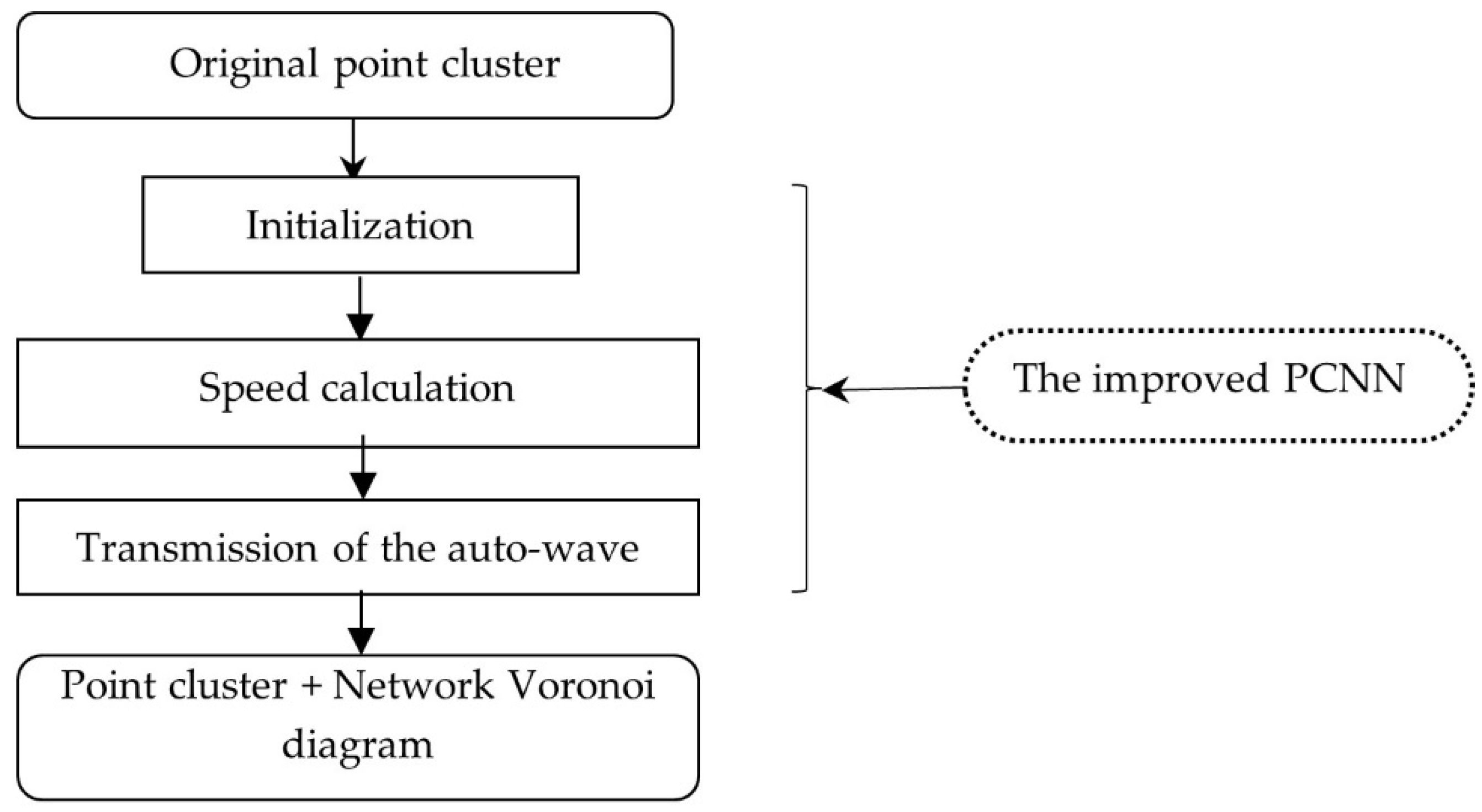
The concrete steps of the construction can be concluded as: Firstly, the initialization is down so that all facility points can be projected onto the related road segments. Secondly, the projected points act as initial neurons in the improved PCNN, and generate auto-wave simultaneously. The speed of auto-wave is calculated and then the auto-wave transmits along the shortest path between neurons. Finally, the road segments conquered by a specific auto-wave and their related space are identified as its initial neuron’s impacting region. Until all the nodes are fired, the network Voronoi diagram of corresponding facility points is successfully generated. The flowchart of the algorithm is shown in Figure 4, and the following describes the procedure in detail.
As shown in Figure 4, the new algorithm includes three procedures:
- − Initialization;
- − Speed calculation;
- − Transmission of the auto-wave.
4.1. Initialization
On the map, the points do not exactly lie on the road segments because the roads are usually represented as lines. In order to match the points with the road segments, the initialization of the improved PCNN model includes points’ projection and the establishment of the connection relationship matrix between neurons.
4.1.1. Points’ Projection
The first step of the algorithm is projecting all the points in the point cluster onto the road segments, aiming at locating the positions of initial neurons (points in the point cluster) on the road network in the improved PCNN model. As shown in Figure 5, perpendiculars from points P1–P5 to the nearest road segments are able to be found. The intersection (marked as P1′–P5′) between the perpendiculars and the road segments can be regarded as the projection of the points.
4.1.2. Connection Relationship Matrix between Neurons
The key of the algorithm is that the auto-waves emitted from different points broadcast along the shortest path between neurons. In order to find the shortest path between neurons, the connection relationship matrix, which stores the distances between neurons, should be constructed at first, as shown in Formula (12).
where n is the total number of the neurons. The weight between neuron i and j is denoted as wij, which assigns the length of the road if there is connection between neuron i and j, or infinity if there is no connection between neuron i and j.
4.2. Transmission of the Auto-Wave
After initialization, the auto-wave will be generated from the initial neurons and then transmit along the shortest distance from the current neuron to the next neuron. In this procedure, the transmission speed of the auto-wave is computed based on the importance of initial neurons and attributes of road segments. The speed needs to be calculated at first, and then transmission will be done.
4.2.1. Speed Calculation
In real traffic networks, some roads are one-way and some roads are two-way, which play different roles in the transportation system. Similarly, the facilities themselves also have different importance with respect to different functions, which can affect the impacting regions of facilities. Therefore, these factors should be considered while computing transmission speed. For instance, the auto-wave will transmit quicker to compete for a larger growth area if it is generated from an important point and expand along an important road. These impact factors are illustrated specifically as follows:
- Direction of the roads
The auto-wave can only expand along the road if its expanding direction is the same as the direction of the road. Otherwise, the transmission of the auto-wave should be terminated. For example, if the road merely permits moving from west to east, the auto-wave expanding from east to west must stop on this road. This can be expressed by Formula (13):
where DR is the direction factor of the current road segment. F (N1, N2) is a direction function which equals to 1 if the auto-wave is the same as the direction of the road and equals to 0 otherwise.
- Grades of the roads
As we all know, the traffic capacities of roads are different. Generally, a road of a higher grade has a higher traffic capacity, and the auto-wave can transmit quicker along these kinds of roads correspondingly. Formula (14) is defined to represent the differences:
where GR is grade factor of the current road segment, and function W(R) denotes the grade function of the road segment.
- Grades of the points
The higher the grade of a point is, the larger its impact range, which can be represented as Formula (15):
where GP is the grade factor of the current point, and function W(N) denotes the importance of the initial neuron.
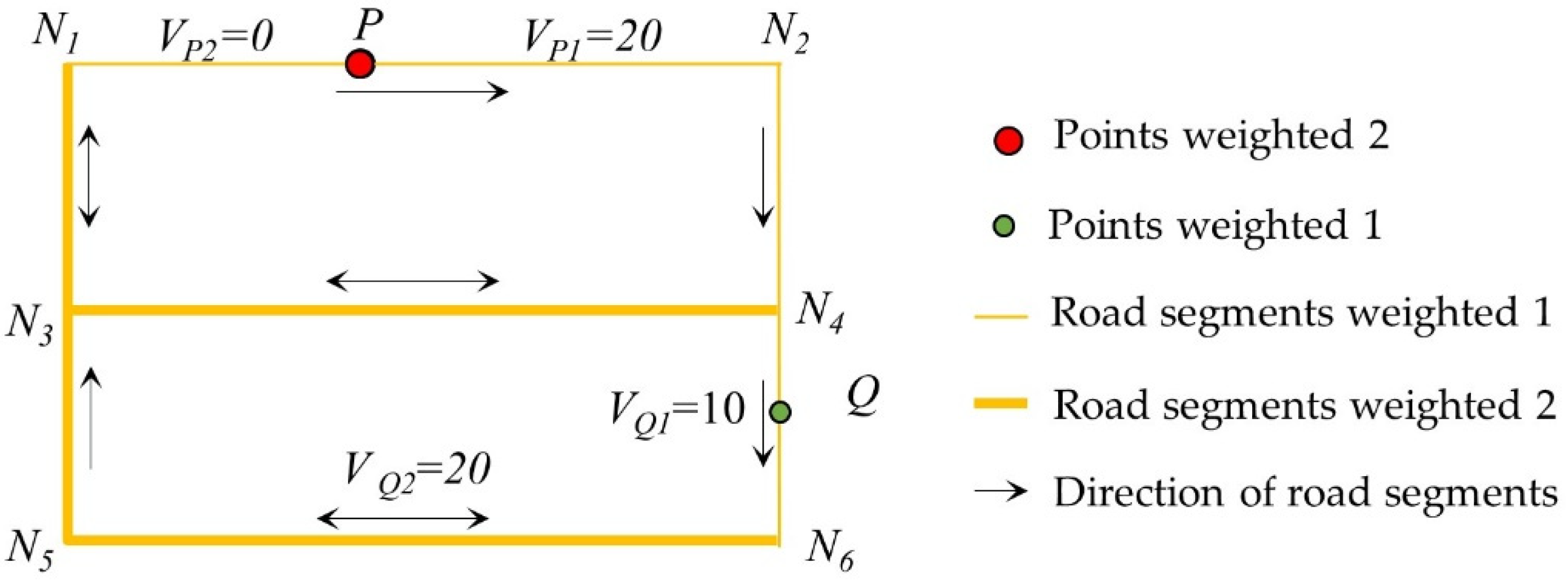
By considering all above factors, the transmitting speed can be defined as Formula (16), where k is the speed of the auto-wave which is generated from initial neurons, weight 1, and transmits along the road segment of weight 1.
As shown in Figure 6, if the unit speed of the auto-wave (generated by neurons of weight 1 and expanding on the road segment of weight 1) is set as 10 m per iteration, the speed of the auto-wave generated from point P is 20 m per iteration (Vp1) when expanding along road segment PN2, and 0 m per iteration (Vp2) when expanding along road segment PN1. VQ1 (the speed of the auto-wave generated from point Q and expanding along road segment QN6) is 10 m per iteration, and VQ2, which represents the speed on road segment N6N5, is 20 m per iteration.
4.2.2. Transmission of the Auto-Wave
In the improved PCNN, the auto-wave which is generated simultaneously by initial neurons will expand along the shortest path between neurons with the above-calculated speed, until all the neurons are fired and the transmitting auto-wave stops. The concrete steps are described as follows:
- (1)
- Initialization of networks’ parameters
The initial iteration number is set as n = 0. The projected points in point cluster and all the nodes in road network are regarded as neurons, and the projected points are chosen as initial neurons (bm) whose initial state is set to be fired (Ybm [0] = 1). The initial neurons are regarded as the mother neurons of other neurons (par(p) = bm). VE is a constant satisfying condition: VE > (n − 1) Wmax, in which N is the total number of the neurons, and Wmax represents the maximum value of the connection weight between neurons. The initial dynamic threshold of iteration is set as EP [0] = VE, YP [0] = 0, S [0] = 0, △S [0] = 0.
- (2)
- Operation of the improved PCNN
Step1: Dynamic threshold of iteration (EP[n]) is calculated by the Formula (8).
Step2: The transmission speed of the auto-wave (LBn) is updated according to Formula (16), and the current wave velocity is set as △S[n] = LBn.
Step3: The current wavelength is calculated by Formula (9) as: S[n] = S[n − 1] + △S[n].
Step4: The current dynamic threshold (EP[n]) is compared with the current wavelength (S[n]). If S[n] ≥ EP[n], then YP[n] = 1, which means neuron P is fired successfully in the nth iteration. Otherwise, YP[n] = 0 and the current neuron P is not fired yet.
Step5: The connection weight Wqp[n + 1] is updated by Formula (11).
Step6: Turn to step 1 to repeat the above steps, until all the neurons are fired and the transmitting auto-wave stops.
The initial state of the points and the road network is shown as Figure 7a. If the weights of the point and the road segments are ignored, which means all the points have the same importance and all the road segments are two-way and have the same importance, the end state of auto-wave transmission is shown as Figure 7b. When the weights of the points and the road networks are all considered and the auto-wave transmits with different speed on different road segments, the end state is shown in Figure 7c. In Figure 7c, the auto-wave generated from the projection points expands along road segments at the speed calculated by Formula (9). It will transmit along the shortest path between neurons until all the neurons are fired. In Figure 7b,c, the black dotted lines represent the road segments which were not passed by the auto-wave. The appearance of this type of road segment is because the auto-wave travels along the shortest path between neurons in the improved PCNN. As soon as the neurons ahead are fired (i.e., the shortest path toward the current neurons is found already), the current auto-wave that travels toward them will stop. For example, in Figure 7c, the auto-wave generated from point P3′ (marked in purple) stops at point r2, because at that very moment the neuron ahead of the auto-wave (r2) is fired by another auto-wave (marked in red). In the end, r1 r2 is the road segment that is never reached by any auto-wave. This kind of road segment is assigned to two initial neurons if the two nodes of the road segment are fired by auto-waves generated from two initial neurons (r1 r2 for example). Otherwise, the road segments are assigned to the only initial neurons (r3 r4 for example). According to this method, these untouched road segments are assigned to the corresponding neurons, and the result is as shown in Figure 8. It can be seen that the road segments (marked in different color) and the corresponding space are assigned to different points.
4.3. The Construction of the Weighted Network Voronoi Diagram
As described above, the construction of the weighted network Voronoi diagram can be summarized as the following steps:
- (1)
- Preprocess the network data: ① All the nodes are found and regarded as the neurons in the improved PCNN, and the road network is divided by the nodes into road segments. ② The point cluster is projected onto the road segments, and the projection points are set as initial neurons. ③ The connection relationship matrix between neurons is computed.
- (2)
- Perform transmission based on the improved PCNN: The auto-waves generated from the initial neurons expand along the corresponding road segments with the speed calculated by the Formula (9); they look for and travel along the shortest paths between neurons simultaneously. The auto-wave will not stop until all the neurons ahead have been fired.
- (3)
- Repeat (2) until all the neurons are fired and the transmitting auto-waves stop.
- (4)
- Road segments that are not used by any auto-wave are assigned to the corresponding initial neurons. So far, the road network and the corresponding space are assigned to the initial neurons and the weighted network Voronoi diagram has been constructed.
As shown in Figure 8, the network space is distributed to different points according to the weights of the points and the attribution of the road segments by the shortest path principle.
5. Experiment Studies and Discussion
5.1. Experiments
To illustrate the soundness of the proposed algorithm, experiments were conducted on the data of a district in a big city, which consists of 2820 road segments (50 national highways, 44 provincial ways, 892 urban first-grade ways, 1834 urban second-grade ways) and 148 educational institutions in three grades. The initial state is shown in Figure 9a. The state at the beginning of the auto-wave transmission is shown as Figure 9b, in which the auto-waves generated from different initial neurons are marked in different colors. Figure 9c shows the final state of auto-wave transmission, where the road segments that are not traveled along by the auto-waves are assigned to the corresponding initial neurons. Finally, the weighted network Voronoi diagram is generated as shown in Figure 9d.
For comparison, experiments using ordinary weighted Voronoi diagram were performed on the same point cluster (Figure 10).
5.2. Discussion
It can be seen in Figure 9d and Figure 10 that: (1) the ordinary weighted Voronoi diagram cut the network planar smoothly, and the weighted network Voronoi diagram cut the network planar unevenly, for the road network is usually unevenly distributed and there is a slight chance to connect original facility points by a straight line. (2) The ordinary weighted Voronoi diagram ignores the influence of the road network where the point cluster is located; thus, the final results would be the same even if the point cluster were put into different road networks. However, the weighted network Voronoi diagram is constructed while fully considering the attributes of road networks, and the importance of points, which ends up providing results more suitable to real life. (3) The weighted network Voronoi diagram is close to the ordinary weighted Voronoi diagram when the road network around the point is dense enough. For instance, the shaded areas (A in Figure 9d and A′ in Figure 10), which represent the impacting regions of the same points calculated by the two methods, are similar in both shape and size, due to the large density of the road network related to the point. If the following three assumptions stand—(1) the road network density is large enough and any two facility points can be connected by roads similar to straight lines, (2) all the roads in road network are of the same weight and (3) all the roads in road network are two-way—it can be inferred that the weighted network Voronoi diagram will be nearly the same as the ordinary weighted Voronoi diagram. However, in fact, the road networks are usually unevenly distributed, and different roads in road network always have different attributes, such as grades and directions. Therefore, it is doubtless that the weighted network Voronoi diagram is a better choice for the representation of the impact scope of a point cluster rather than the ordinary weighted Voronoi diagram.
A comparison experiment based on the idea of the shortest path was performed on the same data. The weighted network Voronoi diagram was constructed using the tool SANET (http://sanet.csis.u-tokyo.ac.jp/), as shown in Figure 11b. It can be deducted that the method based on the idea of the shortest path ignores some of influence factors, such as the attributes of the related road networks. For instance, the road segments next to the points P1 and P2 are of higher grade in Figure 11a, so the auto-waves transmit faster along them, resulting in larger impacting regions of P1 and P2 than in Figure 11b. In addition, as shown in Table 1, experiments with different unit speed were performed, and performance parameters of the proposed algorithm for constructing weighted network Voronoi diagrams are described in Table 1. It can be seen that the iteration number is directly related to the transmission speed of the auto-wave, which can be adjusted according to the practical situation. It can be seen that the time complexity of the algorithm mainly depends on the transmission speed of the auto-wave in the improved PCNN, which is able to be adjusted according to the attributes of the point cluster and the related road network to meet the requirements of accuracy and efficiency. For example, the unit speed of the auto-wave can be set a larger value if the average distance between neurons is small, or a smaller value if the higher accuracy is demanded.
6. Conclusions
This paper proposed an algorithm with which to generate weighted network Voronoi diagrams based on improved PCNN. Experiments showed that: (1) owing to the idea of parallel processing and shortest path transmission of the improved PCNN, the construction process is intuitive and conforms to the basic ideas of the original Voronoi diagram but with a different distance metric. (2) The influences of the point cluster and the related road network are taken into account as weights in the computation, and the constructed weighted network Voronoi diagram can better define the boundaries of the service region of the corresponding point.
The improved PCNN and the algorithm can also be extended to linear facilities and polygon facilities; and it will be our future work to introduce more semantic information into the construction, based on which, the weighted network Voronoi diagram for linear and polygon facilities will be constructed.
Author Contributions
X.L. and H.Y. proposed the methodology. X.L. performed the experiments and wrote the draft of the manuscript. H.Y. guided the research and revised the manuscript. All the authors contributed to the development of the proposed generalization algorithm and this manuscript. All authors have read and agreed to the published version of the manuscript.
Funding
This research was funded by the National Nature Science Foundation of China, grant numbers 42161066 and 41801395, and the Nature Science Foundation of Gansu province, grant number 20JR10RA246.
Institutional Review Board Statement
Not applicable.
Informed Consent Statement
Informed consent was obtained from all subjects involved in the study.
Data Availability Statement
Not applicable.
Acknowledgments
The authors are grateful to anonymous reviewers, whose comments and suggestions have helped us to improve the context and presentation of the article.
Conflicts of Interest
The authors declare no conflict of interest.
References
- Gold, C.M. Review: Spatial Tessellations-Concepts and Applications of Voronoi Diagrams. Int. J. Geogr. Inf. Sci. 1994, 8, 237–238. [Google Scholar]
- Dumic, E.; Bjelopera, A.; Nüchter, A. Dynamic Point Cloud Compression Based on Projections, Surface Reconstruction and Video Compression. Sensors 2022, 22, 197. [Google Scholar] [CrossRef] [PubMed]
- Huang, S.-K.; Wang, W.-J.; Sun, C.-H. A Path Planning Strategy for Multi-Robot Moving with Path-Priority Order Based on a Generalized Voronoi Diagram. Appl. Sci. 2021, 11, 9650. [Google Scholar] [CrossRef]
- Polianskii, V.; Pokorny, F.T. Voronoi Graph Traversal in High Dimensions with Applications to Topological Data Analysis and Piecewise Linear Interpolation. In Proceedings of the KDD’20: The 26th ACM SIGKDD Conference on Knowledge Discovery and Data Mining, Virtual Event, 6–10 July 2020. [Google Scholar]
- Zhao, X.; Chen, J.; Wang, J. O-QTM based Algorithm for the Generating of Voronoi Diagram for Spherical Objects. Acta Geod. Cartogr. Sin. 2002, 31, 158–163. [Google Scholar]
- Okabe, A.; Satoh, T.; Furuta, T.; Suzuki, A.; Okano, K. Generalized Network Voronoi Diagrams: Concepts, Computational Methods and Applications. Int. J. Geogr. Inf. Sci. 2008, 22, 965–994. [Google Scholar] [CrossRef]
- Randazzo, G.; Cascio, M.; Fontana, M.; Gregorio, F.; Lanza, S.; Muzirafuti, A. Mapping of Sicilian Pocket Beaches Land Use/Land Cover with Sentinel-2 Imagery: A Case Study of Messina Province. Land 2021, 10, 678. [Google Scholar] [CrossRef]
- Lage, M.d.O.; Machado, C.A.S.; Monteiro, C.M.; Davis, C.A., Jr.; Yamamura, C.L.K.; Berssaneti, F.T.; Quintanilha, J.A. Using Hierarchical Facility Location, Single Facility Approach, and GIS in Carsharing Services. Sustainability 2021, 13, 12704. [Google Scholar] [CrossRef]
- Kiani, F.; Seyyedabbasi, A.; Nematzadeh, S.; Candan, F.; Çevik, T.; Anka, F.A.; Randazzo, G.; Lanza, S.; Muzirafuti, A. Adaptive Metaheuristic-Based Methods for Autonomous Robot Path Planning: Sustainable Agricultural Applications. Appl. Sci. 2022, 12, 943. [Google Scholar] [CrossRef]
- Ai, T.; Yu, W. Algorithm for Constructing Network Voronoi Diagram Based on Flow Extension Ideas. Acta Geod. Cartogr. Sin. 2013, 42, 760–766. [Google Scholar]
- Ai, T.; Yu, W.; He, Y. Generation of constrained network Voronoi diagram using linear tessellation and expansion method. Comput. Environ. Urban Syst. 2015, 51, 83–96. [Google Scholar] [CrossRef]
- Liu, F.; Andrienko, G.; Andrienko, N.; Chen, S.; Janssens, D.; Wets, G.; Theodoridis, Y. Citywide Traffic Analysis Based on the Combination of Visual and Analytic Approaches. J. Geovisualization Spat. Anal. 2020, 4, 15. [Google Scholar] [CrossRef]
- Harn, P.; Zhang, J.; Shen, T.; Wang, W.; Jiang, X.; Ku, W.-S.; Sun, M.-T.; Chiang, Y.-Y. Multiple ground/aerial parcel delivery problem: A Weighted Road Network Voronoi Diagram based approach. Distrib. Parallel Databases 2021, 1–21. [Google Scholar] [CrossRef]
- Gotoh, Y.; Okubo, C. A proposition of querying scheme with network Voronoi diagram in bichromatic reverse k-nearest neighbor. Int. J. Pervasive Comput. Commun. 2017, 13, 62–75. [Google Scholar] [CrossRef]
- Xie, S.; Feng, X.; Du, J. Maximal Covering Spatial Optimization Based on Network Voronoi Diagrams Heuristic and Swarm Intelligence. Acta Geod. Cartogr. Sin. 2011, 40, 778–784. [Google Scholar]
- Tu, W.; Li, Q.; Fang, Z. Large Scale Multi-depot Logistics Routing Optimization Based on Network Voronoi Diagram. Acta Geod. Cartogr. Sin. 2014, 43, 1075–1082. [Google Scholar]
- Miller, H.J. Market Area Delimitation within Networks Using Geographic Information Systems. Geogr. Syst. 1994, 1, 157–173. [Google Scholar]
- Tan, Y.; Zhao, Y.; Wang, Y. Power network Voronoi diagram and dynamic construction. J. Netw. 2012, 7, 675–682. [Google Scholar] [CrossRef] [Green Version]
- Grumbly, S.M.; Frazier, T.G.; Peterson, A.G. Examining the Impact of Risk Perception on the Accuracy of Anisotropic, Least-Cost Path Distance Approaches for Estimating the Evacuation Potential for Near-Field Tsunamis. J. Geovisualization Spat. Anal. 2019, 3, 3. [Google Scholar] [CrossRef]
- Chen, J. A Raster-based Method for Computing Voronoi Diagrams of Spatial Objects Using Dynamic Distance Transformation. Int. J. Geogr. Inf. Sci. 1999, 13, 209–225. [Google Scholar] [CrossRef]
- Zhao, R.; Li, Z.; Chen, J.; Gold, C.M.; Zhang, Y. A Hierarchical Raster Method for Computing Voronoi Diagrams Based on Quadtrees. In Computational Science—ICCS 2002; Lecture Notes in Computer Science Computational Science-ICCS; Springer: Amsterdam, The Netherland, 2002; pp. 85–92. [Google Scholar]
- Deng, X.; Yang, Y.; Zhang, H.; Ma, Y. PCNN double step firing mode for image edge detection. Multimed. Tools Appl. 2022, 1–15. [Google Scholar] [CrossRef]
- Yang, G.; Lu, Z.; Yang, J.; Wang, Y. An adaptive contourlet HMM–PCNN model of sparse representation for image denoising. IEEE Access 2019, 7, 88243–88253. [Google Scholar] [CrossRef]
- Basar, S.; Waheed, A.; Ali, M.; Zahid, S.; Zareei, M.; Biswal, R.R. An efficient Defocus Blur Segmentation Scheme Based on Hybrid LTP and PCNN. Sensors 2022, 22, 2724. [Google Scholar] [CrossRef] [PubMed]
- Shen, Y.; Yuan, Y.; Peng, J. Research on Near Infrared and Color Visible Fusion Based on PCNN in Transform Domain. Spectrosc. Spec. Anal. 2021, 41, 2023. [Google Scholar]
- Sun, Y.; Yang, H. Path Planning Based on Pulse Coupled Neural Networks with Directed Constraint. Comput. Sci. 2019, 46, 28–32. [Google Scholar]
- Eckhorn, R.; Reitboeck, H.J.; Arndt, M.; Dicke, P.W. A neural network for feature linking via synchronous activity: Result from cat visual cortex and from simulation. In Models of Brain Function; Cambridge University Press: Cambridge, UK, 1989; pp. 255–272. [Google Scholar]
- Gao, C.; Zhou, D.; Guo, Y. An Iterative Thresholding Segmentation Model Using a Modified Pulse Coupled Neural Network. Neural Process. Lett. 2014, 39, 81–95. [Google Scholar] [CrossRef]
- Zhao, T.; Wang, J.; Zhang, J. Real-time multimodal transport path planning based on a pulse neural network model. Int. J. Simul. Process Model. 2017, 12, 356. [Google Scholar] [CrossRef]
- Johnson, J.L. Pulse-coupled neural networks. In Neural Networks and Pattern Recognition; Academicpp: San Diego, CA, USA, 1998; pp. 1–56. [Google Scholar]
- Li, B.; Zhao, K.; Sandoval, E.B. A UWB-Based Indoor Positioning System Employing Neural Networks. J. Geovisualization Spat. Anal. 2020, 4, 18. [Google Scholar] [CrossRef]
Figure 1.
An example of the planar Voronoi diagram.

Figure 2.
Structure of the PCNN model.

Figure 3.
Structure of the improved PCNN.

Figure 4.
Flowchart of the algorithm.

Figure 5.
Projection of the points.

Figure 6.
The speed of the auto-wave under constraints.

Figure 7.
Transmission of auto-waves.

Figure 8.
The final state of auto-wave transmission.

Figure 9.
The generation of the weighted network Voronoi diagram of points in the study area.

Figure 10.
Weighted Voronoi diagram of points in the study area.

Figure 11.
A comparison between the weighted network Voronoi diagram using the model of improved PCNN and that based on the idea of the shortest path.
Figure 11.
A comparison between the weighted network Voronoi diagram using the model of improved PCNN and that based on the idea of the shortest path.


Table 1.
Performance parameters of the algorithm for constructing weighted network Voronoi diagrams.
Table 1.
Performance parameters of the algorithm for constructing weighted network Voronoi diagrams.
| Experiment | Unit Speed of the Auto-Wave (m) | Number of Iterations | Construction Time(s) |
|---|---|---|---|
| Figure 9 | 1 | 1323 | 9.3 |
| 5 | 321 | 2.1 |
Publisher’s Note: MDPI stays neutral with regard to jurisdictional claims in published maps and institutional affiliations. |
© 2022 by the authors. Licensee MDPI, Basel, Switzerland. This article is an open access article distributed under the terms and conditions of the Creative Commons Attribution (CC BY) license (https://creativecommons.org/licenses/by/4.0/).
Share and Cite
MDPI and ACS Style
Lu, X.; Yan, H. An Algorithm to Generate a Weighted Network Voronoi Diagram Based on Improved PCNN. Appl. Sci. 2022, 12, 6011. https://doi.org/10.3390/app12126011
AMA Style
Lu X, Yan H. An Algorithm to Generate a Weighted Network Voronoi Diagram Based on Improved PCNN. Applied Sciences. 2022; 12(12):6011. https://doi.org/10.3390/app12126011
Chicago/Turabian StyleLu, Xiaomin, and Haowen Yan. 2022. "An Algorithm to Generate a Weighted Network Voronoi Diagram Based on Improved PCNN" Applied Sciences 12, no. 12: 6011. https://doi.org/10.3390/app12126011
Note that from the first issue of 2016, this journal uses article numbers instead of page numbers. See further details here.