Optimizing Voronoi-based quantifications for reaching interactive analysis of 3D localizations in the million range
 Florian Levet1,2*
- 1CNRS, Interdisciplinary Institute for Neuroscience, IINS, UMR 5297, University of Bordeaux, Bordeaux, France
- 2CNRS, INSERM, Bordeaux Imaging Center, BIC, UAR3420, US 4, University of Bordeaux, Bordeaux, France
Over the last decade, single-molecule localization microscopy (SMLM) has revolutionized cell biology, making it possible to monitor molecular organization and dynamics with spatial resolution of a few nanometers. Despite being a relatively recent field, SMLM has witnessed the development of dozens of analysis methods for problems as diverse as segmentation, clustering, tracking or colocalization. Among those, Voronoi-based methods have achieved a prominent position for 2D analysis as robust and efficient implementations were available for generating 2D Voronoi diagrams. Unfortunately, this was not the case for 3D Voronoi diagrams, and existing methods were therefore extremely time-consuming. In this work, we present a new hybrid CPU-GPU algorithm for the rapid generation of 3D Voronoi diagrams. Voro3D allows creating Voronoi diagrams of datasets composed of millions of localizations in minutes, making any Voronoi-based analysis method such as SR-Tesseler accessible to life scientists wanting to quantify 3D datasets. In addition, we also improve ClusterVisu, a Voronoi-based clustering method using Monte-Carlo simulations, by demonstrating that those costly simulations can be correctly approximated by a customized gamma probability distribution function.
Introduction
SMLM has induced a major paradigm shift from conventional light microscopy modalities: SMLM datasets are composed of the precise coordinates, in 2D or 3D, of the molecules being acquired. As pixel-based analysis methods were not adapted, these point clouds have required the development of a whole new set of analysis tools based on geometry and spatial organization (Khater et al., 2020). Among those, Voronoi-based methods have emerged as one of the standard in the field, whether it be for clustering (Andronov et al., 2016), segmentation (Levet et al., 2015; Peters et al., 2017) or colocalization (Levet et al., 2019; Ejdrup et al., 2022) and motion (Beheiry. et al., 2015) analysis.
Nevertheless, the rapid adoption of SMLM by life scientists has highlighted an important limitation of existing analysis methods. As datasets composed of millions of localizations are now routinely acquired in biology labs and facilities, it has become obvious that very few methods were capable of scaling to this magnitude, and that especially in 3D. This results in the necessity to define small ROIs composed of 104–105 localizations for analysis, as quantifying a whole dataset in one go is out of reach. For instance, and while 3D analysis with Voronoi diagrams is available for a few years now, it takes several hours to quantify datasets in the 1.106 localization range (Andronov et al., 2018). This unfortunately lacks the interactivity required when analyzing an unknown biological model, as life scientists may need to fine-tune their analysis parameters through several attempts.
In this paper, we propose to optimize two Voronoi-based quantification methods for segmentation and clustering, SR-Tesseler (Levet et al., 2015) and ClusterVisu (Andronov et al., 2016; Andronov et al., 2018), to make them interactive for analyzing 3D SMLM datasets in the millions range. Our contributions are twofold. First, we have developed a new hybrid CPU-GPU algorithm (called Voro3D) for the rapid generation of 3D Voronoi diagrams. Voro3D allows constructing diagrams composed of millions of localizations in a few minutes, achieving state of the art timing for heterogeneous point clouds. Second, we have shown that clustering can be performed without requiring the use of costly Monte Carlo simulations (Andronov et al., 2016; Andronov et al., 2018), as the cell size distribution of randomly placed localizations can be approximated by an analytical function. All these developments are available in our newly released PoCA platform (Levet and Sibarita, 2023).
Methods
3D Voronoi diagram generation
Voronoi diagram is a well-known space-subdividing technique used in dozens of different domains (Atsuyuki et al., 2003) that also met great success in the context of SMLM (Beheiry. et al., 2015; Levet et al., 2015; Andronov et al., 2016; Peters et al., 2017; Andronov et al., 2018; Levet et al., 2019; Ejdrup et al., 2022). Depending on the application, it can be generated with or without its global combinatorial information (i.e., the global mesh geometry) using a variant of the Bower-Watson (Bowyer, 1981; Watson, 1981) or Lloyd (Lloyd, 1982) algorithms. As expected, algorithms generating the global combinatorial information are costlier, thus necessitating access to CPU clusters (Chrisochoides and Nave, 2003; González, 2016) or machines with large number of cores (CGAL, 2020), two equipment that may be out of reach for most biology labs. On the other hand, and when this combinatorial information is unnecessary, each Voronoi cell can be computed individually without requiring synchronization of the global geometry. In this case, each cell only requires to gather its direct neighbors to be generated. Algorithms based on this idea combine supervised spatial subdivisions (subdivision techniques requiring a user-defined parameter for gathering neighbors) with parallelization (Rycroft, 2009; Ray et al., 2018) to speed up the computation speed (Figure 1A). Nevertheless, these implementations are based on the assumption that the originating point clouds are evenly distributed, i.e., that their spatial distribution is homogeneous, which is in general not the case for SMLM data. In Ray et al. (2018), the authors managed to create 3D Voronoi diagrams of millions of points in a few seconds on the GPU. This impressive result was achieved by retrieving the k-closest neighbors of each point with a kd-tree, and by using them to brute force the Voronoi cell construction. Nevertheless, this implies that the k-nearest neighbors surrounding a point represent a proper sampling of its vicinity, a hypothesis that is only certified in the case of a homogeneous distribution combined with a sufficient number of neighbors (Figure 1A top).
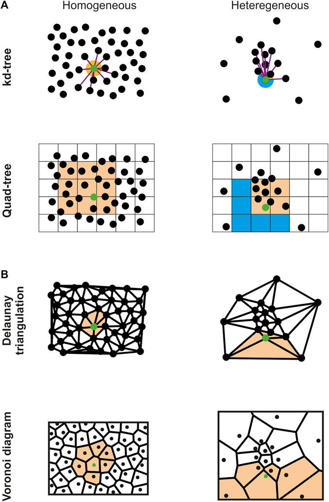
FIGURE 1. Comparison of the vicinity sampling of a specific point (green) with different spatial subdivision techniques and distributions. (A) Supervised spatial subdivision techniques (kd-tree, n = 10; quad-tree, side = 25) properly sample the point vicinity (orange) in the homogeneous case (left) but fail to correctly capture some region of the vicinity (blue) for heterogeneous distributions (right). (B) On the contrary, unsupervised techniques (Delaunay triangulation and Voronoi diagram) properly sample the point vicinity (orange) for both homogeneous and heterogeneous distributions.
To adapt this process to inhomogeneous point cloud data, we used the Delaunay triangulation, which is the dual of the Voronoi diagram, to compute the Voronoi diagram (Algorithm 1). We integrated a very efficient CPU implementation available in the CGAL (2020) library, that allows computing a 3D Delaunay diagram of 10 million of localizations in around 10 s with a standard computer. Using the connectivity provided by the Delaunay triangulation, all the direct neighbors pn of a given point p, i.e., the points part of the tetrahedrons originating from p, can be efficiently retrieved. Contrary to the k-nearest neighbors, pn is guaranteed to accurately describe the vicinity of p in all directions (Figure 1B top). We then modified the algorithm provided in (Ray et al., 2018) to brute force the Voronoi diagram construction on the GPU using pn (Figure 1B bottom), allowing creating the 3D Voronoi diagrams of inhomogeneous SMLM point cloud data composed of millions of localizations in a few minutes. Implementation discrepancies between CGAL and the GPU code (Ray et al., 2018) forced us to develop a function gathering all the localizations’ direct neighbors in an array (Algorithm 1 line 2). In addition, the Voronoi cells are not returned in (Ray et al., 2018) since their application only required to compute the cells volume, a feature for which it is unnecessary to explicitly create the cells. Consequently, we added a CPU function to create the Voronoi cells from the convex hull of the cells’ points (Barber et al., 1996).
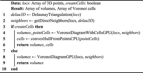
Algorithm 1. Voro3D pseudocode.
Voronoi-based clustering
To perform statistical clustering, Andronov et al. compared experimental SMLM datasets with Monte Carlo simulations (Andronov et al., 2016; Andronov et al., 2018) (Figure 2). They generated a user-defined number of simulations having the same number of localizations and volume but exhibiting a random spatial distribution (Figures 2A, B). By comparing the cell size distribution (i.e., volume for three dimensional datasets) of the experimental dataset with the mean cell size distribution of all the simulations, they were able to automatically determine a threshold to segment clusters (Figures 2C, D). Their technique has a strong limitation: as their implementation of the 3D Voronoi diagram was not optimized, and since the global computation time linearly scales with the number of simulations, 3DClusterVisu took up to 6 h for analyzing datasets in the 1.106 localizations range.
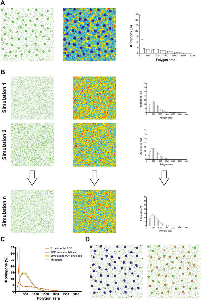
FIGURE 2. ClusterVisu method. (A) Clustered simulation exhibiting 20 clusters (left) with corresponding Voronoi diagram (middle) and cell size distribution (right). (B) Simulations of randomly placed points (left) having the same density and area of the clustered simulation with corresponding Voronoi diagrams (middle) and cell size distributions (right). (C) Threshold (green) is identified as the intersection between the cell size distribution of the clustered simulation (red) and the mean of the cell size distributions of all the random simulations (blue), with the envelope being displayed in orange. (D) Corresponding Voronoi cells selection (left) and clusters (right).
Voronoi diagrams of random spatial distributions are called Poisson Voronoi diagrams and have been extensively studied (Hermann et al., 1989; Kumar et al., 1992; Masaharu, 2003; Ferenc and Néda, 2007; Hinde and Miles, 2007; Zaninetti, 2009; González and Einstein, 2011). Of particular interest is the cell size distribution
with a and c two shape parameters and b a scale parameter. From all the proposed distributions, we used the ones from Ferenc and Néda (2007):
The error between the cell size distribution of simulated datasets and this analytical distribution has been quantified to be less than 0.04% and 1%, for 2D and 3D, respectively (Ferenc and Néda, 2007).
Nevertheless, blinking of the molecules is not taken into account by this numerical approximation. Monte Carlo simulations, on the other hand, should be able to integrate this blinking behavior in the cell size distribution, as long as the simulator provides a realistic simulation of blinking, a task known to be difficult. Another difference between the numerical approximation and Monte Carlo simulations is the cell size distribution envelope provided by running several simulations (Figure 2C). This envelope helps to assess how much an experimental dataset deviates from a random distribution of points. Another potential solution to quantify this deviation is to compute the Ripley’s functions (Ripley, 1977; Nieves et al., 2023).
Results
Voro3D is available in our newly released SMLM analysis platform called PoCA (Levet and Sibarita, 2023). While PoCA is developed in C++ and can therefore be executed on any computer, Voro3D is implemented in Cuda (Nickolls et al., 2008) and therefore requires a computer equipped with a Nvidia graphics card (https://www.nvidia.com/). To our knowledge, the only two libraries implementing 3D Voronoi diagrams for heterogeneous point clouds that are directly accessible are SciPy (Virtanen et al., 2020) (Supplementary Material) and CGAL (2020), which was included in one of our precedent software platform (Levet et al., 2019). We therefore compared the execution time of Voro3D versus SciPy and CGAL for datasets exhibiting a random spatial distribution and ranging from 103 to 107 localizations (Figure 3A). Voro3D is consistently faster than the other two solutions. It achieves generating a 3D Voronoi diagram from a dataset composed of 10 million localizations in close to 1 min and a half, a time suitable with an interactive analysis. Importantly, the implementation of Voro3D available in PoCA takes longer as more operations are performed. In addition to the three steps of the pseudocode (Algorithm 1), there are two additional steps pertaining to computational operations performed on the Delaunay triangulation and the Voronoi diagram, such as computation of the tetrahedra volume or creation of the OpenGL rendering buffers (Figure 3B). Time ratio between the different steps shows the extreme efficiency of both the Delaunay triangulation generation (multithreaded on the CPU, 10.4 s for 10 million localizations) and the construction of the Voronoi cells (GPU, 1.55 s for 10 million localizations). Most of the time is spent on operations performed on CPU without multithreading (92%), such as computational operations on the Delaunay triangulation (43%) or gathering the direct neighbors for the Voronoi cell construction (45%). Finally, the Voronoi GPU code (Ray et al., 2018) computes the Voronoi cells as a combination of tetrahedra, i.e., Voronoi cells are not explicitly constructed and returned. We therefore added an optional function to compute the Voronoi cells based on the convex hull (Barber et al., 1996) (Algorithm 1). This function is time consuming as it is single-threaded and non-optimized (Figure 3C).
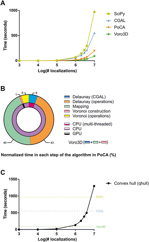
FIGURE 3. Comparison of timings for different algorithms. (A) Comparison of timings for SciPy, CGAL, PoCA and Voro3D for datasets ranging from 1,000 to 10,000,000 localizations. (B) Normalized timings for each step of the 3D Voronoi diagram generation implemented in PoCA. (C) Timings for computing the convex hull of the Voronoi cells for datasets ranging from 1,000 to 10,000,000 localizations. For comparison, the timings for generating the 3D Voronoi diagram for 10,000,000 localizations with Scipy (dark yellow), CGAL (blue) and Voro3D (green) are plotted.
While Voro3D already greatly improves the computation time of 3DClusterVisu (15 min with Voro3D versus 6 h for the original 3DClusterVisu (Andronov et al., 2018) for a dataset composed of 780,000 localizations), using an analytical function approximating the cell size distribution eliminates any additional computational time. Therefore, to demonstrate that Eq. 2 is a good approximation for 3DClusterVisu (Andronov et al., 2018) we first generated a simulated dataset composed of 20 clusters (Figure 4A, referred as experimental), and then computed fifty Monte Carlo simulations having the same localization density but with a random spatial distribution (referred as simulations). The cell volume probability distribution function (PDF) of experimental and simulations were both normalized to be comparable with the analytical PDF (Figures 4B, C). Importantly, we also removed Voronoi cells that were on the border of the dataset volume (i.e., they were cut by the dataset bounding volume) to prevent any edge effect. We found that the simulations and analytical PDFs were not significantly different (Figure 4B, Wilcoxon rank test p-value = 0.1211), a property that also transfers to the computed thresholds (Figure 4C, Tsimulations = 0.307, Tanalytical = 0.312). Finally, objects created with these thresholds exhibited similar shapes and volumes (Figures 4D, E) and their volume distributions were not significantly different (Kolmogorov-Smirnov test p-value = 0.818). We also compared the volume of each object in the simulations with its counterpart in the analytical and quantified the mean difference to be less than 1%. Finally, we also compared clustering between Monte-Carlo simulations and Eq. 2 on an experimental dataset of Xenopus laevis nuclear pore complexes stained with WGA-ATTO520 (Löschberger, 2021) available for download on ShareLoc (Ouyang et al., 2022) (Figure 5A). Similarly to the simulations, the number of segmented clusters is very similar (ClusterVisu, n = 1,108; Eq. 2, n = 1,112; Figure 5B) and their distributions of volume are not significantly different (Kolmogorov-Smirnov test p-value = 0.788, Figure 5C).
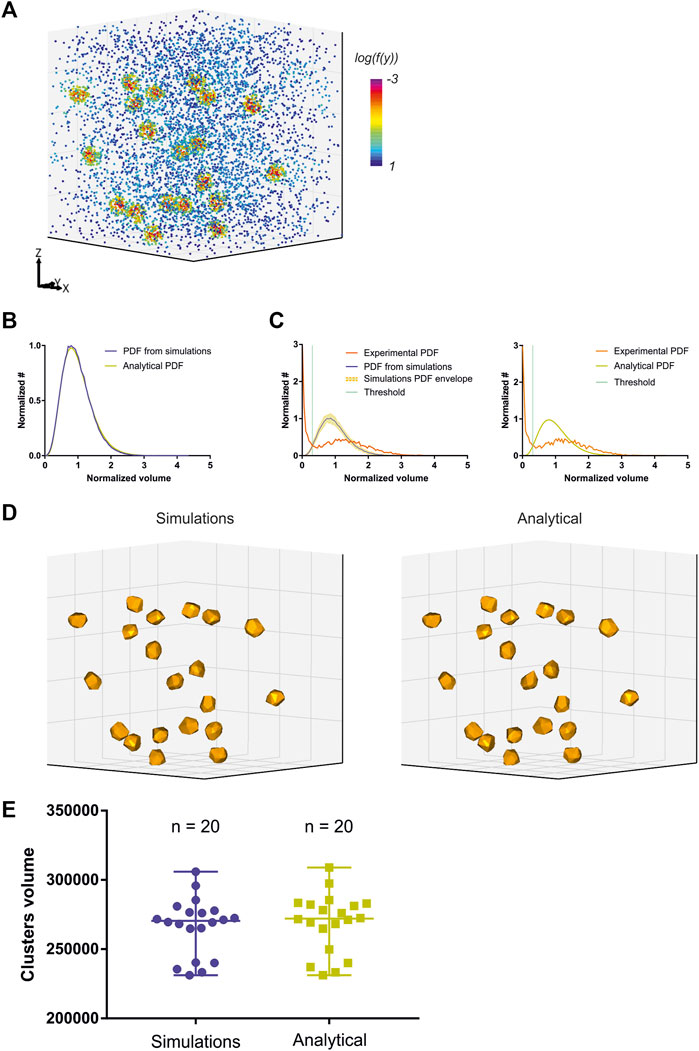
FIGURE 4. Comparison of clustering with Monte-Carlo simulations and a customized gamma distribution on simulations. (A) Simulation of a 3D dataset exhibiting 20 clusters. (B) Comparison of the distribution of normalized Voronoi cells volume between Monte-Carlo simulations (blue) and Eq. 2 (dark yellow). (C) Computed threshold (green) with Monte-Carlo simulations (left) and Eq. 2 (right). (D) Segmented clusters with Monte-Carlo simulations (left) and Eq. 2 (right). (E) Comparison of the segmented cluster volumes with Monte-Carlo simulations (blue) and Eq. 2 (dark yellow).
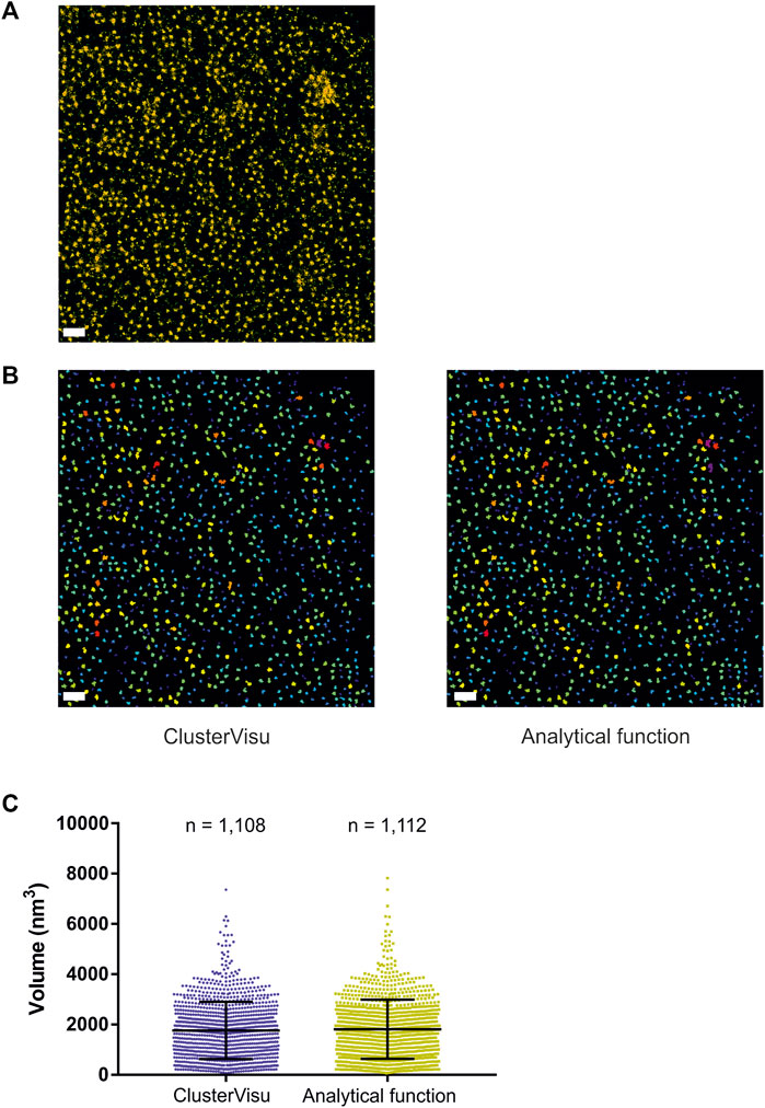
FIGURE 5. Comparison of clustering with Monte-Carlo simulations and a customized gamma distribution on an experimental dataset. (A) Localization dataset of Xenopus laevis nuclear pore complexes stained with WGA-ATTO520, scale bar = 500 nm. (B) Segmented clusters obtained with ClusterVisu (left) and Eq. 2 (right), scale bar = 500 nm. (C) Comparison of the segmented cluster volumes with Monte-Carlo simulations (blue) and Eq. 2 (dark yellow).
Discussion
As 3D SMLM is increasingly adopted by biology labs by ways of imaging facilities, the bottleneck has shifted from not having the technology to image to not being able to analyze and extract meaningful quantifications from the acquired datasets. In the context of 2D SMLM analysis, Voronoi diagrams has become a method of reference (Levet et al., 2015; Andronov et al., 2016; Peters et al., 2017; Andronov et al., 2018; Levet et al., 2019) thanks in part to its rapidity that gave life scientists interactive feedbacks on quantifications. Unfortunately, 3D Voronoi analysis was extremely time-consuming, preventing its use for datasets composed of millions of 3D localizations.
In this paper, we presented a novel hybrid CPU-GPU algorithm called Voro3D for the fast computation of 3D Voronoi diagrams. This algorithm achieves state of the art computation time for point clouds exhibiting heterogeneous spatial distribution. While its implementation in PoCA is slightly more computationally expensive, it is still compatible with an interactive analysis. Voro3D also improves the computation time of any method based on Voronoi diagrams, such as ClusterVisu (Andronov et al., 2016; Andronov et al., 2018). Nevertheless, we also demonstrated that the main component of ClusterVisu, the cell size probability distribution function, can be correctly approximated by a customized gamma distribution. This results in the capability of computing clustering of SMLM datasets with no other additional cost than the Voronoi diagram computation.
From the three steps of the Voro3D algorithm, inspection of the computation time has shown that the majority of the computation time is spent on transferring the localizations’ neighbors from the Delaunay triangulation to the Voronoi diagram (Delaunay computation: 12%, transferring neighbors: 86%, Voronoi computation: 2%). This transfer step is currently required because of discrepancies between the CGAL and Cuda implementations. Multi-threading this step could reduce even more the Voro3D computation time. Similarly, construction of the Voronoi cells is currently time consuming as it is a single-thread CPU process. Constructing the cell at the same time than the tetrahedral decomposition happening in the GPU could massively improve its computation time.
Voro3D is natively included in PoCA and our implementation of ClusterVisu (with Monte Carlo simulations and our analytical approximation) is available as a PoCA’s plugin.
Data availability statement
Publicly available datasets were analyzed in this study. This data can be found here: https://zenodo.org/record/7182237.
Author contributions
FL developed the software, made the figures and wrote the manuscript.
Funding
This work was supported by the Ministère de l’Enseignement Supérieur et de la Recherche (ANR-20-CE11-0006 NANO-SYNATLAS), the Centre National de la Recherche Scientifique (CNRS), the Conseil Régional d’Aquitaine and the Institut National de la Santé et de la Recherche Médicale (Inserm). We also acknowledge France-BioImaging infrastructure supported by the French National Research Agency (ANR-10-INBS-04).
Conflict of interest
The author declares that the research was conducted in the absence of any commercial or financial relationships that could be construed as a potential conflict of interest.
Publisher’s note
All claims expressed in this article are solely those of the authors and do not necessarily represent those of their affiliated organizations, or those of the publisher, the editors and the reviewers. Any product that may be evaluated in this article, or claim that may be made by its manufacturer, is not guaranteed or endorsed by the publisher.
Supplementary material
The Supplementary Material for this article can be found online at: https://www.frontiersin.org/articles/10.3389/fbinf.2023.1249291/full#supplementary-material
References
Andronov, L., Michalon, J., Ouararhni, K., Orlov, I., Hamiche, A., Vonesch, J. L., et al. (2018). 3DClusterViSu: 3D clustering analysis of super-resolution microscopy data by 3D voronoi tessellations. Bioinformatics 34, 3004–3012. doi:10.1093/bioinformatics/bty200
Andronov, L., Orlov, I., Lutz, Y., Vonesch, J., and Klaholz, B. P. (2016). ClusterViSu, a method for clustering of protein complexes by Voronoi tessellation in super-resolution microscopy. Nat. Publ. Gr. 6, 24084–24089. doi:10.1038/srep24084
Atsuyuki, O., Barry., B., Kokichi, S., and Sung Nok, C. (2003). Spatial tessellations: Concepts and applications of Voronoi diagrams. Hoboken: Wiley.
Barber, C. B., Dobkin, D. P., and Huhdanpaa, H. (1996). The quickhull algorithm for convex hulls. ACM Trans. Math. Softw. 22, 469–483. doi:10.1145/235815.235821
Beheiry., M. E., Dahan, M., and Masson, J. B. (2015). InferenceMAP: Mapping of single-molecule dynamics with bayesian inference. Nat. Methods 2015 127 (12), 594–595. doi:10.1038/nmeth.3441
Bowyer, A. (1981). Computing dirichlet tessellations. Comput. J. 24, 162–166. doi:10.1093/comjnl/24.2.162
Chrisochoides, N., and Nave, D. (2003). Parallel Delaunay mesh generation kernel. Int. J. Numer. Methods Eng. 58, 161–176. doi:10.1002/nme.765
Ejdrup, A. L., Lycas, M. D., Lorenzen, N., Konomi, A., Herborg, F., Madsen, K. L., et al. (2022). A density-based enrichment measure for assessing colocalization in single-molecule localization microscopy data. Nat. Commun. 2022 131 (13), 4388–4410. doi:10.1038/s41467-022-32064-y
Enderlein, G., Hogg, R. V., and Craig, A. T. (1961). Introduction to mathematical statistics. The macmillan company, New York, 1 Print 1959, 245 seiten, $ 6,75. Biom. Z. 3, 145–146. doi:10.1002/bimj.19610030210
Ferenc, J. S., and Néda, Z. (2007). On the size distribution of Poisson Voronoi cells. Phys. A Stat. Mech. its Appl. 385, 518–526. doi:10.1016/j.physa.2007.07.063
González, D. L., and Einstein, T. L. (2011). Voronoi cell patterns: Theoretical model and applications. Phys. Rev. E. 84, 051135. doi:10.1103/PhysRevE.84.051135
González, R. E. (2016). Paravt: Parallel Voronoi tessellation code. Astron. Comput. 17, 80–85. doi:10.1016/j.ascom.2016.06.003
Hermann, H., Wendrock, H., and Stoyan, D. (1989). Cell-area distributions of planar Voronoi mosaics. Metallography 23, 189–200. doi:10.1016/0026-0800(89)90030-x
Hinde, A. L., and Miles, R. E. (2007). Monte Carlo estimates of the distributions of the random polygons of the voronoi tessellation with respect to a Poisson process. Taylor Francis group 10, 205–223. doi:10.1080/00949658008810370
Khater, I. M., Nabi, I. R., and Hamarneh, G. (2020). A review of super-resolution single-molecule localization microscopy cluster analysis and quantification methods. Patterns 1, 100038. doi:10.1016/j.patter.2020.100038
Kumar, S., Kurtz, S. K., Banavar, J. R., and Sharma, M. G. (1992). Properties of a three-dimensional Poisson-voronoi tesselation: A Monte Carlo study. J. Stat. Phys. 67, 523–551. doi:10.1007/bf01049719
Levet, F., et al. (2015). SR-tesseler: A method to segment and quantify localization-based super-resolution microscopy data. Nat. Methods 12. doi:10.1038/nmeth.3579
Levet, F., Julien, G., Galland, R., Butler, C., Beghin, A., Chazeau, A., et al. (2019). A tessellation-based colocalization analysis approach for single-molecule localization microscopy. Nat. Commun. 10, 2379–2412. doi:10.1038/s41467-019-10007-4
Levet, F., and Sibarita, J.-B. (2023). PoCA: A software platform for point cloud data visualization and quantification. Nat. Methods 20, 1–2. doi:10.1038/s41592-023-01811-4
Lloyd, S. P. (1982). Least squares quantization in PCM. IEEE Trans. Inf. Theory 28, 129–137. doi:10.1109/tit.1982.1056489
Löschberger, A. (2021). Xenopus laevis nuclear pore complex stained with WGA-ATTO520. doi:10.5281/ZENODO.7182237
Masaharu, T. (2003). Statistical distributions of Poisson Vorono¨ı cells in two and three dimensions.
Nickolls, J., Buck, I., Garland, M., and Skadron, K. (2008). Scalable parallel programming with CUDA. Queue 6, 40–53. doi:10.1145/1365490.1365500
Nieves, D. J., Pike, J. A., and Levet, F. (2023). A framework for evaluating the performance of SMLM cluster analysis algorithms. Nat. Methods 2023 202 (20), 259–267. doi:10.1038/s41592-022-01750-6
Ouyang, W., Bai, J., and Singh, M. K. (2022). ShareLoc — An open platform for sharing localization microscopy data. Nat. Methods 2022 1911 (19), 1331–1333. doi:10.1038/s41592-022-01659-0
Peters, R., Benthem Muñiz, M., Griffié, J., Williamson, D. J., Ashdown, G. W., Lorenz, C. D., et al. (2017). Quantification of fibrous spatial point patterns from single-molecule localization microscopy (SMLM) data. Bioinformatics 33, 1703–1711. doi:10.1093/bioinformatics/btx026
Ray, N., Sokolov, D., Lefebvre, S., and Lévy, B. (2018). Meshless voronoi on the GPU. ACM Trans. Graph. 37, 1–12. doi:10.1145/3272127.3275092
Ripley, B. D. (1977). Modelling spatial patterns. J. R. Stat. Soc. Ser. B 39, 172–192. doi:10.1111/j.2517-6161.1977.tb01615.x
Rycroft, C. H. (2009). VORO++: A three-dimensional voronoi cell library in C++. Chaos Interdiscip. J. Nonlinear Sci. 19 (4), 041111. doi:10.1063/1.3215722
Virtanen, P., Gommers, R., and Oliphant, T. E. (2020). SciPy 1.0: Fundamental algorithms for scientific computing in Python. Methods 2020 173 (17), 261–272. doi:10.1038/s41592-019-0686-2
Watson, D. F. (1981). Computing the n-dimensional Delaunay tessellation with application to Voronoi polytopes. Comput. J. 24, 167–172. doi:10.1093/comjnl/24.2.167
Keywords: single molecule localisation microscopy (SMLM), segmentation, Voronoi–Delaunay tessellation, GPU (CUDA), clustering
Citation: Levet F (2023) Optimizing Voronoi-based quantifications for reaching interactive analysis of 3D localizations in the million range. Front. Bioinform. 3:1249291. doi: 10.3389/fbinf.2023.1249291
Received: 28 June 2023; Accepted: 27 July 2023;
Published: 04 August 2023.
Edited by:
Hannah S. Heil, Gulbenkian Institute of Science (IGC), PortugalReviewed by:
Leonid Andronov, Stanford University, United StatesKoen Martens, University of Bonn, Germany
Copyright © 2023 Levet. This is an open-access article distributed under the terms of the Creative Commons Attribution License (CC BY). The use, distribution or reproduction in other forums is permitted, provided the original author(s) and the copyright owner(s) are credited and that the original publication in this journal is cited, in accordance with accepted academic practice. No use, distribution or reproduction is permitted which does not comply with these terms.
*Correspondence: Florian Levet, florian.levet@u-bordeaux.fr